Abstract
This solo-author preprint studies cheap online diagnostics for grokking phase regimes in transformers. The public artifact includes a Python package, aggregate JSONs, provenance manifests, figure artifacts, Lean 4 checks, and a Hugging Face dataset.
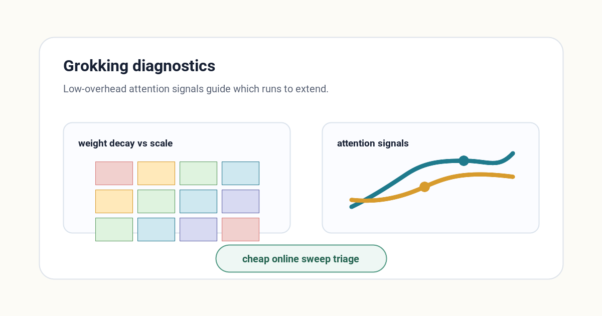
TL;DR: Two cheap statistics computed directly from attention weights track when and whether a transformer "groks" a task, at about 3% extra compute cost. Across 1,120 runs we map a phase diagram over weight decay and model size, and show the critical weight-decay threshold is architecture-specific, not a universal constant.
If you're skimming
- Question: can we see grokking phase behavior without expensive second-order diagnostics?
- Diagnostics: attention-head cosine similarity and entropy spread across heads.
- Scale: 1,120 transformer runs for the main regime map, plus 350 cross-architecture probes.
- Limit: the critical weight-decay threshold is architecture-specific, so the number should not be copied blindly.
What "grokking" means here
Train a small transformer on a synthetic task like modular addition and something strange happens: the model first memorizes the training examples, the training loss drops to near zero, and test accuracy stays low, sometimes for thousands of steps. Then, seemingly out of nowhere, test accuracy jumps and the model generalizes. That delayed jump is called grokking.
Knowing whether and when a run will grok matters if you're studying generalization, but the standard ways to detect the underlying phase transition (Hessian-based diagnostics) are expensive to compute during training.
The two cheap diagnostics
We compute two numbers directly from the model's attention activations during training:
- Mean pairwise attention-head cosine similarity (written s̄) - how similar the attention heads are to each other.
- Entropy standard deviation across heads (written σH) - how much the heads disagree in how spread-out their attention is.
Both track the grokking phase regime from attention activations alone, at roughly 3% wall-clock overhead in the reported setting, complementing the more expensive Hessian-based diagnostics at much lower compute cost.
How to read the figure
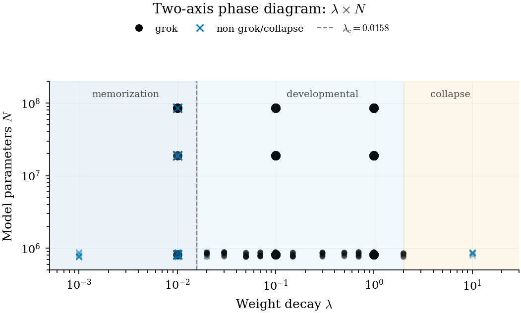
The x-axis is weight decay and the y-axis is model scale. The point of the figure is not that one region is "good" and the others are "bad." It is a map of training behavior: too little regularization leaves you in memorization, an intermediate region supports delayed generalization, and too much regularization can push the run into collapse.
The useful part is operational. If you are launching a sweep, the figure tells you that weight decay is not a single knob with a universal setting. The same value can mean different things after model scale changes.
The regime map
Across the 1,120 runs, we map a 2-axis regime diagram (weight decay × model size). The critical weight decay for the canonical 4-layer, 8-head, 128-dimension transformer on modular addition lands at λc ≈ 0.0158, with a power-law exponent ν ≈ 0.757 describing how the transition sharpens with scale.
What I would use this for
I would use these diagnostics as cheap sweep instrumentation, not as a final theorem about grokking. They are useful when you need to decide whether to extend a run, kill a run, or sample more densely near a suspected transition. Because they come from attention activations, they can run during training without the cost of a full Hessian-style probe.
The strongest use case is early triage: if a sweep is expensive, I want a low-overhead signal that tells me which runs are worth watching longer. The diagnostic does not replace final test accuracy. It gives a reason to spend the next compute dollar on one part of the grid instead of another.
The architecture-specificity result
We then ran the same diagnostics on three other architectures at matched horizons: a 4-layer MLP, a 4-layer LSTM, and a 4-layer Mamba (selective state-space) model, 350 additional runs. Each showed a different critical weight-decay value: about 0.0511 for the MLP, 0.0365 for the LSTM, and 0.0144 for Mamba. The Mamba value overlaps the transformer's canonical range, but we don't claim that overlap reflects a shared underlying transition mechanism. The practical takeaway is that a critical weight-decay number measured on one architecture should be recalibrated, not assumed to transfer, when you move to a different architecture.
What is public
- Paper on arXiv with the full sweep design and regime analysis.
- GitHub repository with code, manifests, aggregate JSONs, figure artifacts, and Lean checks.
- Hugging Face dataset for the released run artifacts.
Frequently asked questions
What is "grokking" in transformers?
A network first memorizes training data, then, much later, suddenly generalizes to the test set - often long after the training loss looks flat.
What are the two new diagnostics?
Mean pairwise attention-head cosine similarity and entropy standard deviation across heads, both computed straight from attention activations at roughly 3% overhead.
Is the critical weight-decay value the same across architectures?
No. MLP, LSTM, and Mamba each showed a different critical value in our cross-architecture probes. Recalibrate per architecture rather than transferring the transformer number.
Is any of this formally verified?
The diagnostic identities are checked with Lean 4 proofs against mathlib. The empirical claims are separately traced through aggregate JSON provenance, not formally proven.
Links
BibTeX
@article{verma2026grokkingdiagnostics,
  title={Weight Decay Regimes in Grokking Transformers: Cheap Online Diagnostics},
  author={Verma, Lucky},
  journal={arXiv preprint arXiv:2605.20441},
  year={2026}
}